Medical Imaging · 2026
Multi-label chest X-ray classification with DenseNet-121
Detecting 14 pathologies at once in 112,000 chest X-rays, with an asymmetric loss, per-pathology calibrated thresholds and Grad-CAM++ to audit the model.
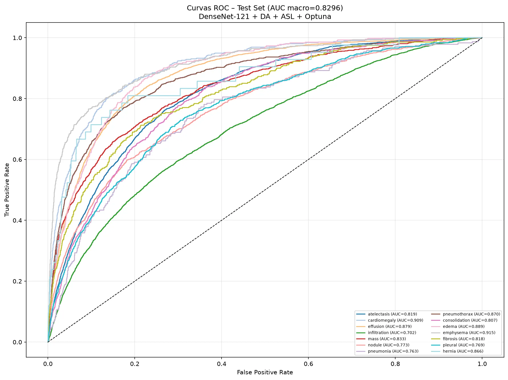
- macro AUC-ROC on test
- 0.83
- pathologies assessed at once on every image
- 14
- chest X-rays in ChestMNIST
- 112,120
- AUC over the MedMNIST v2 ResNet-50 reference
- +0.06
Problem
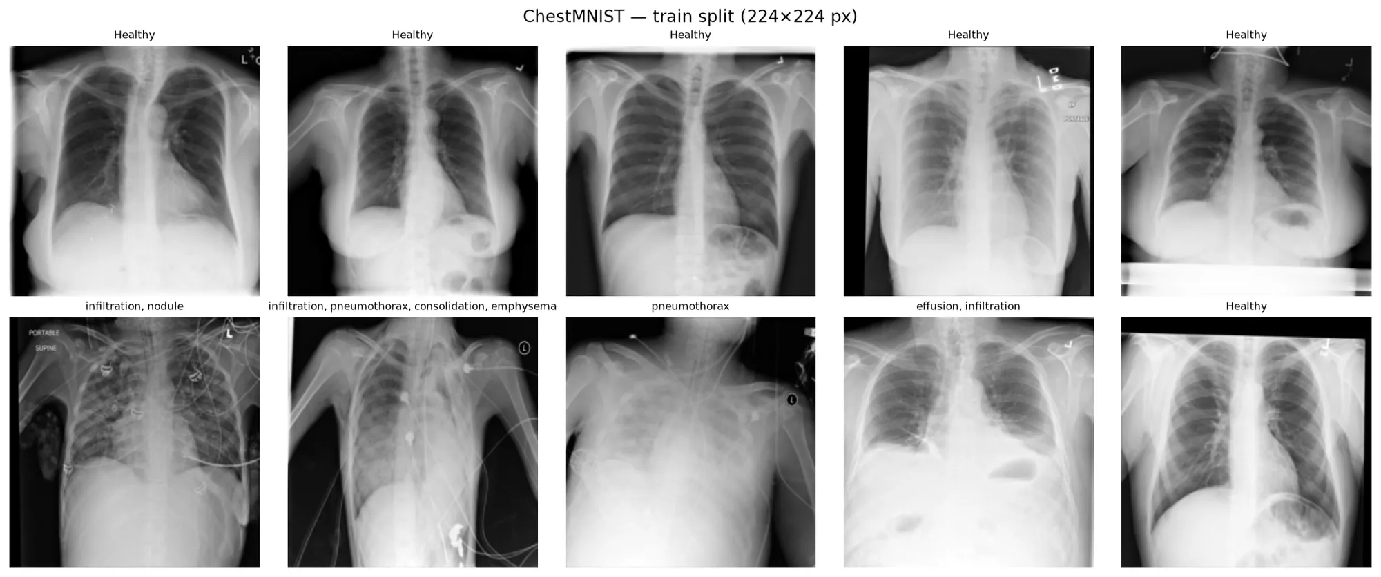
A chest X-ray can show several pathologies at once, or none. ChestMNIST, derived from NIH ChestX-ray14, contains 112,120 X-rays labelled with 14 pathologies: atelectasis, cardiomegaly, effusion, infiltration, mass, nodule, pneumonia, pneumothorax, consolidation, edema, emphysema, fibrosis, pleural thickening and hernia. It is a multi-label problem: for every image, the model decides separately whether each pathology is present.
 View full-size image
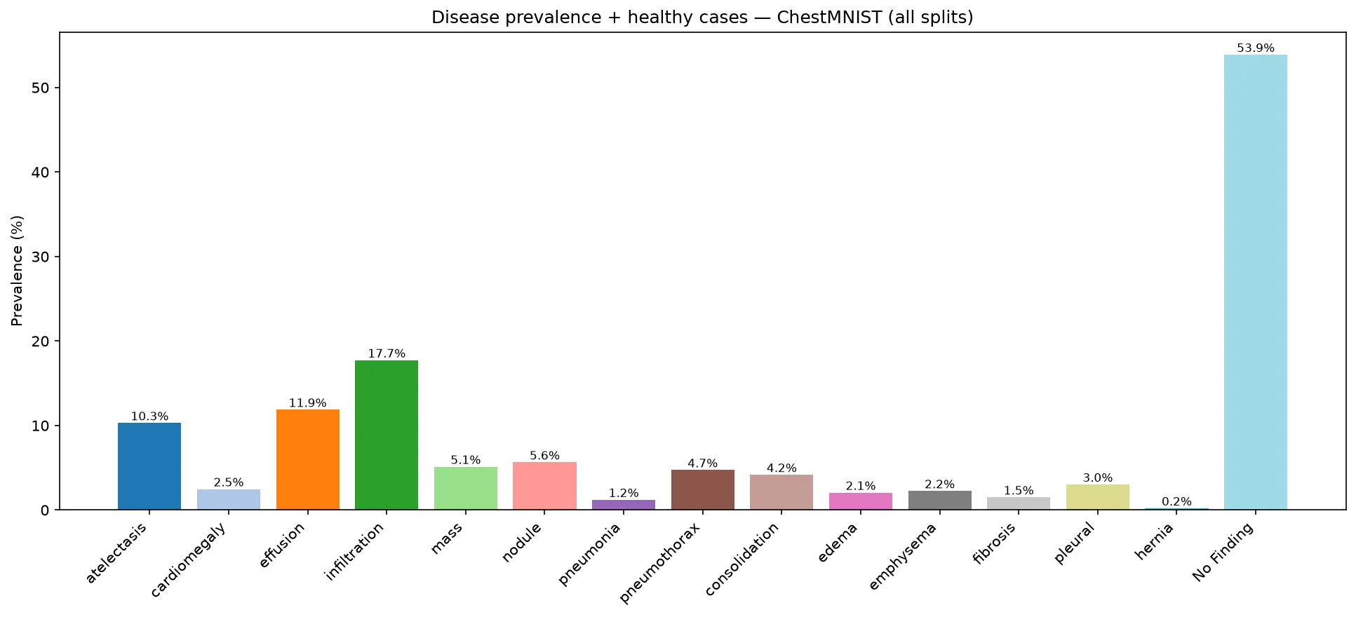
The hard part is the imbalance. 53.9% of the images have no finding and some classes are very rare (hernia: 0.2%). A model that always answers “healthy” gets more than 90% of the labels right and detects nothing. That is why accuracy is not the main metric: the work is evaluated with AUC-ROC, F1 and balanced accuracy.
 View full-size image
My contribution
Solo project for the Pattern Recognition and Machine Learning Applications course:
- Exploratory analysis: label distribution, number of pathologies per image and the effect of resolution.
- An experimental study changing one factor at a time: resolution, loss function, architecture, data augmentation, and full fine-tuning versus a frozen encoder.
- A final pipeline packaged in Python, with one module per stage, paths relative to the project root, timestamped logs and pinned dependencies.
- Per-pathology threshold calibration and explainability with Grad-CAM++.
Technical approach
The baseline is an ImageNet-pretrained ResNet-50 with full fine-tuning, BCE and 224 px input. From there I compared each decision separately and kept what worked:
- Resolution: 224 px beats 128 px (+0.018 AUC). Small findings such as nodules need detail.
- Loss: the Asymmetric Loss (ASL) gives more weight to positives and down-weights easy negatives, which are the vast majority.
- Architecture: DenseNet-121, the same family as CheXNet, performs slightly better than ResNet-50.
- Data augmentation: rotations, translations and horizontal flips with MONAI. It is the single change with the largest effect.
- Fine-tuning: freezing the encoder drops AUC to 0.74. ImageNet features are not enough; the whole network has to adapt to X-rays.
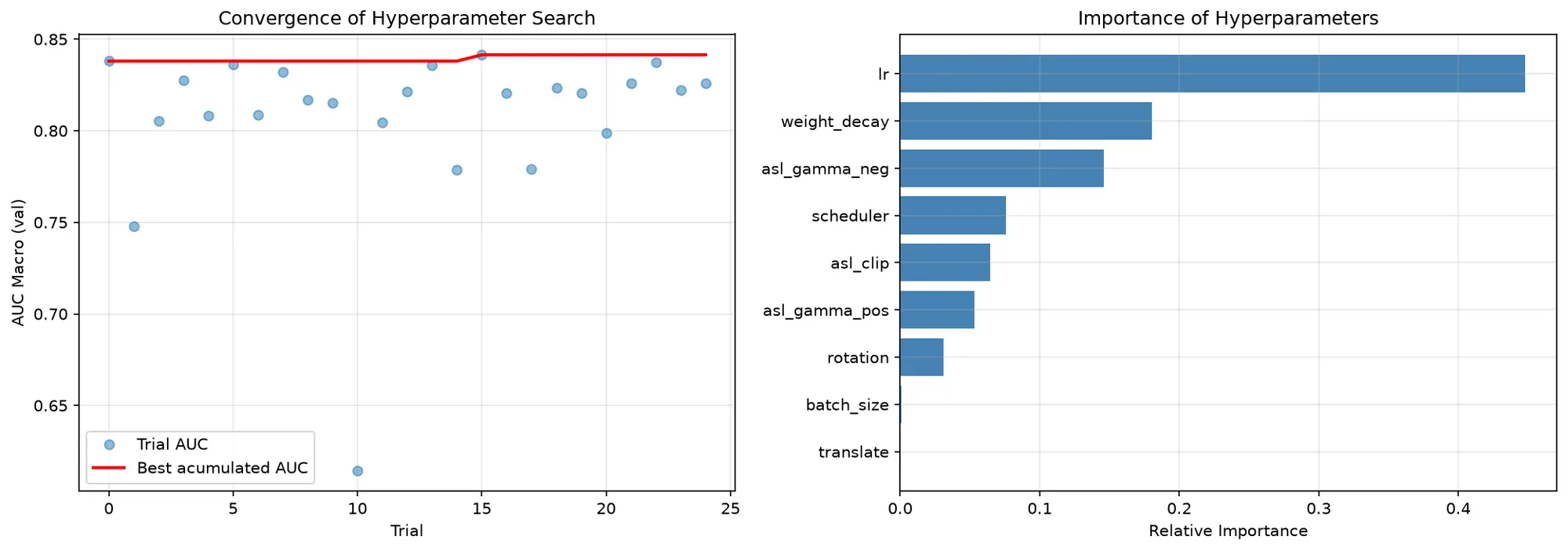
- Hyperparameter searchOptuna: 25 trials with TPE and median pruningval. AUC 0.841
- TrainingDenseNet-121 + ASL + data augmentation, with early stoppingmax. 30 epochs
- Threshold calibrationOne threshold per pathology, chosen on validation among 6 strategies
- Test evaluationAUC, F1, Hamming, exact match and balanced accuracy
- ExplainabilityGrad-CAM++ on the last dense blockdenseblock4
Optuna jointly tunes the learning rate, batch size, weight decay, scheduler, the three ASL parameters and the augmentation strength.
 View full-size image
The asymmetric loss is the core of training. It uses a different γ exponent for positives and negatives and shifts negative probabilities so that the easiest ones are discarded:
# src/models/losses.py — AsymmetricLoss.forward (simplified)
xs_pos = torch.sigmoid(x)
# Shift negatives: very easy ones stop counting
xs_neg = (1 - xs_pos + self.clip).clamp(max=1)
loss = y * torch.log(xs_pos.clamp(min=self.eps)) \
     + (1 - y) * torch.log(xs_neg.clamp(min=self.eps))
pt = xs_pos * y + xs_neg * (1 - y)
# Different γ exponent for positives and negatives
gamma = self.gamma_pos * y + self.gamma_neg * (1 - y)
loss *= torch.pow(1 - pt, gamma)
return -loss.mean()
Results
- ResNet-50 at 128 px0.807
- Baseline: ResNet-50 at 224 px0.825
- Weighted BCE0.817
- Focal loss0.823
- Asymmetric loss0.826
- DenseNet-1210.827
- Data augmentation0.837
- Frozen encoder0.736
- Final pipeline (DenseNet-121 + ASL + augmentation + Optuna)0.830
Scale from 0.70 to 0.85
| Test metric | Baseline | Final pipeline |
|---|---|---|
| Macro AUC-ROC | 0.8245 | 0.8296 |
| Macro F1 | 0.2721 | 0.3075 |
| Exact match (all labels right) | 0.3570 | 0.3901 |
| Hamming score | 0.9102 | 0.9139 |
| Mean balanced accuracy | 0.6513 | 0.6577 |
The final pipeline improves on the baseline mainly in macro F1 (+0.035) and in images with every label right (+3.3 points). In AUC, the best variants are within hundredths of each other, the same gap that separates two runs of the final pipeline itself (0.8296 in the repository run and 0.8361 in the presentation run). With that much variation, the pipeline’s value is not an extra tenth: it is that the whole process is reproducible with a single command.
The result is on par with the state of the art on ChestMNIST: it beats the official MedMNIST v2 references (ResNet-50 at 224 px: 0.773) and approaches what has been reported with foundation models (0.835).
Choosing the threshold is a clinical decision
With 14 probabilistic outputs, you have to decide above which value each pathology counts as present. The code compares six strategies on validation and picks the one with the highest macro F1:
| Strategy (validation) | Macro F1 | Missed cases | False alarms |
|---|---|---|---|
| Youden per pathology | 0.229 | 2,229 | 31,555 |
| Best global threshold (0.38) | 0.269 | 3,570 | 11,359 |
| F1 per pathology (chosen) | 0.314 | 4,056 | 9,376 |
| Fixed threshold 0.5 | 0.204 | 5,943 | 2,416 |
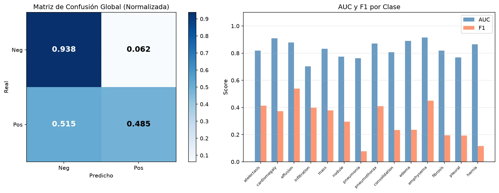
The table shows the trade-off: the fixed 0.5 threshold raises almost no false alarms but misses nearly 6,000 findings. In screening, where a missed case costs more than an extra review, Youden would be the better choice even with a lower F1. That decision belongs with the clinical team; it should not be a default value.
 View full-size image
 View full-size image
Where the model looks
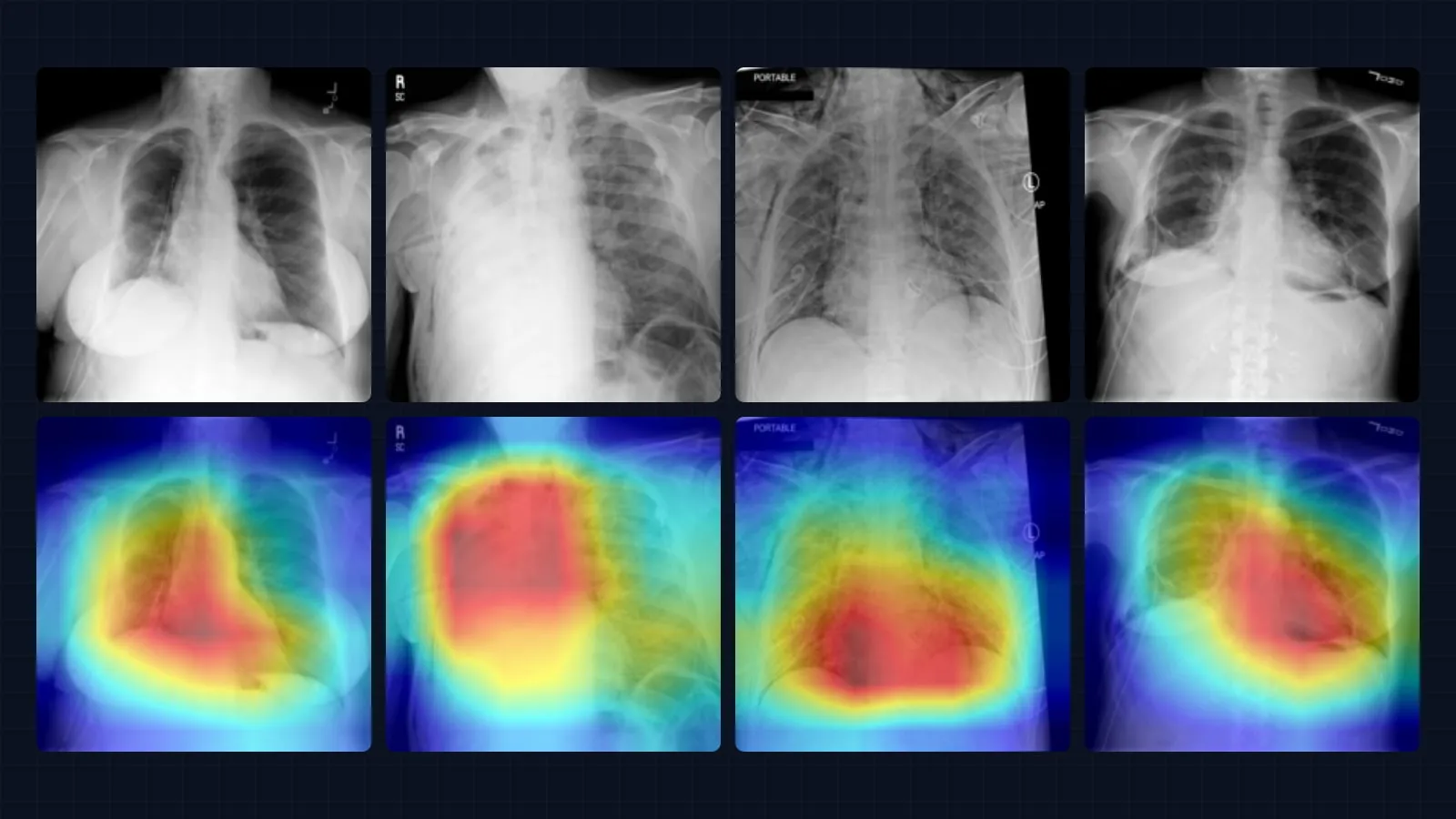
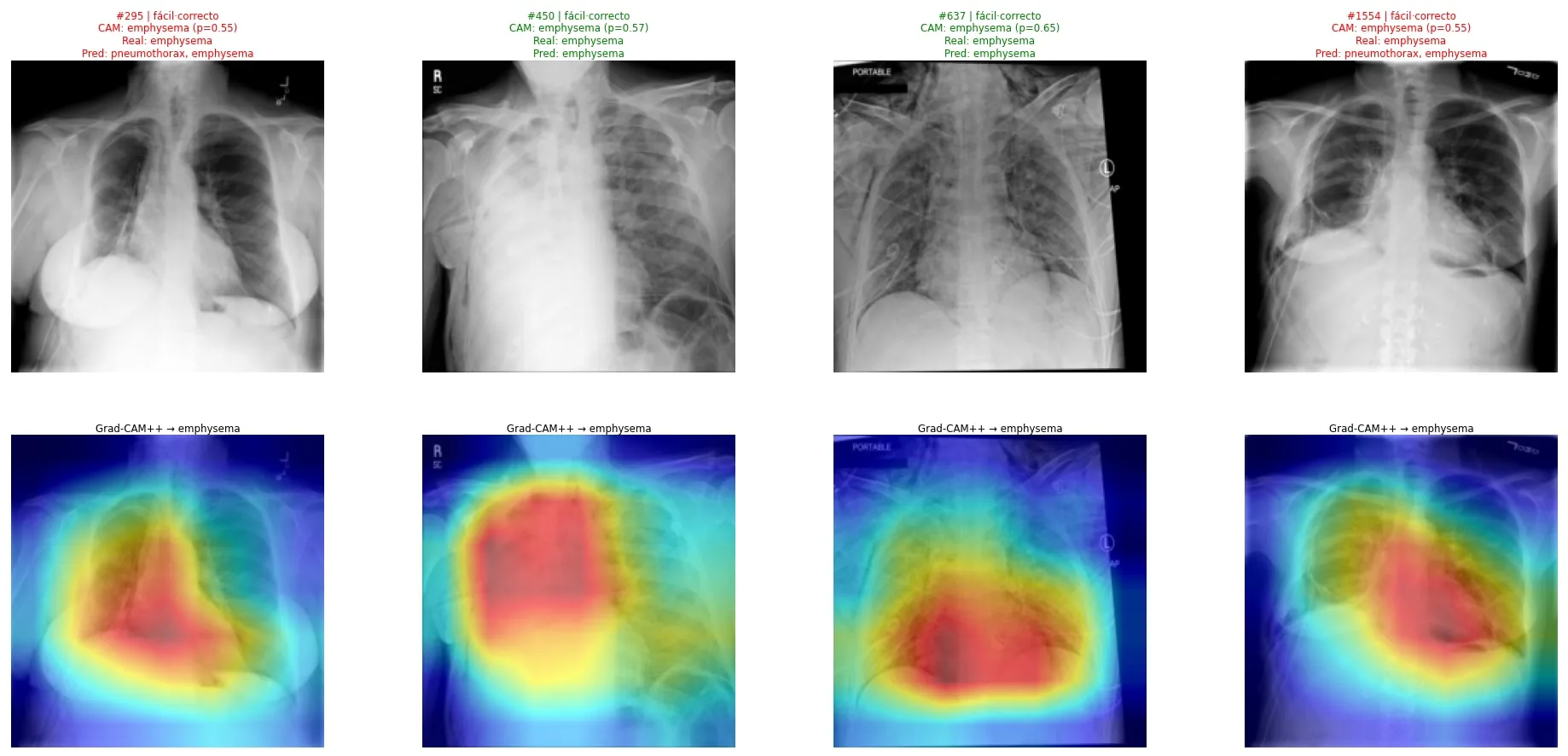
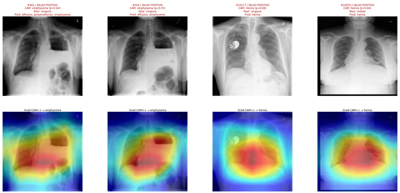
For a given pathology, Grad-CAM++ highlights the image regions that weighed most in the prediction. It is a way to check that the model looks at the lungs and not at markers, cables or text on the film.
 View full-size image
 View full-size image
Limitations:
- F1 for rare classes is still low (pneumonia 0.08; hernia 0.11): with so few positives, any threshold produces many false alarms.
- Each variant was trained once, with one split and one seed. Differences of hundredths are not conclusive.
- ChestX-ray14 labels were mined automatically from radiology reports and are noisy.
- At 224 px it stays below models trained on full-resolution NIH ChestX-ray14 (e.g. 0.853 AUC with a DenseNet-121).
Evidence
- Repository with the code, the logs of every run and the final metrics as JSON (
results/). - Slides with the full study: state of the art, ablations and explainability.
- To reproduce it:
pip install -r requirements.txt && pip install -e ., thenpython -m src.pipelines.pipeline_final.
Professional application
- Multi-label classifiers with imbalanced classes: medical imaging, industrial inspection with several defects per part, or content tagging.
- Setting thresholds from the real cost of each type of error instead of defaulting to 0.5.
- Auditing a vision model with explainability maps before putting it in front of users.
More projects
See all projects
Medical Imaging
Melanoma segmentation with U-Nets built from scratch in PyTorch
Two U-Nets coded from scratch to outline skin lesions: one trained from scratch and one with a frozen pretrained ResNet-50 encoder.
Computer Vision
Ablation study on MNIST and CIFAR-10: 99.47% and 93.87% accuracy
Two ablation studies measuring how much each piece contributes to beating 99.4% on MNIST without convolutions and 92% on CIFAR-10.